
This project does reference to the next github repositories:
HAWC Observatory: datasets
- Mention to Emmanuel Anguiano-Hernández mecanosaurio.
- Introduction
- Reconstruction
- Process
- Methodology
- Rehearsal
- Presentation
- Tools
- Python
- Processing
- References
Each time of second, a certain gamma-ray particles that travels from the interstellar medium to earth's atmosphere, has been cascading our bodies. While we are reading this, perhaps.
At the beginning, these particles comes mostly from cosmic-ray sources, like; kilonovaes, supernovaes, pulsars, stars' collisions or even galaxies' centers. When they hit in the atmosphere, they interact with the atomic nuclei and elementary particles are produced, which turns them into more particles to generate a cascade effect. This showers of particles grows until all the energy of the original gamma-ray is totally used. You might imagine all this happening approximately at 10 km above sea level, and that could cover an area of even a 1,000 of square meters.
So, The High-Altitude Water Cherenkov (HAWC) Gamma-Ray Observatory attends this wonderful research on the flanks of the Sierra Negra volcano on Pico de Orizaba's (Citlaltépetl) National Park, near from the beautiful city of Puebla in México. It implements a 140x180m territorial area, with 300 cylindrical modules of 7.3x4.5m filled with 200,000L of purified water, and three floating photomultiplier tubes (PMT) for each one.
Now, when an elementary particle of the atmosphere cascade travels through the water, it produces a light pulse call Cherenkov radiation. This happens when an electric charged particle travels faster than light in a medium like water. It's similar when at the poles of the planets experiences the auroras borealis or autralis, because of the protection role of the atmosphere from the higher levels of gamma-ray or radiation.

Thereby, the light pulses are detected by a photocathode material of the PMT, which converts and multiply the signal from the photon particle into many electrons, and sends an electrocmagnetic pulse to 1,200 channels from 120 front-end boards in the observatory. The front-end boards processes those pulses into interpretable datasets store onto tabular representations with the information about arrive time and cascade's size.
Finally, through this information and the data from the 2HWC HAWC Observatory Gamma-Ray Catalogue, we intented to figure out the phenomena dimension from its domain to synthesize a qualitive form, that could reveals and amplify cognitive structures of cosmic ray's events into an inferencial pattern system, which allows Astronomers to reconstruct the direction from the original gamma-ray source, and estimates its energy through a based-computer simulation that visualize and sonorize its nature.
For the pictorical and sound reconstructions of the phenomena, we wanna answer some of these questions:
- From where the Gamma-Ray came from?
- How a Gamma-Ray emmited from Crab Nebulae travels to Earth.
- What is a Gamma-Ray cascade?
- How does the modules detect these particles?
- How does this information is create in the machine-system?
- What is the sound representation of all this?
Also, we are interested in explore the quantities of time in nanoseconds (ns) from the cascade events, that allows Astronomers to infer the trajectory angle of the gamma-ray.
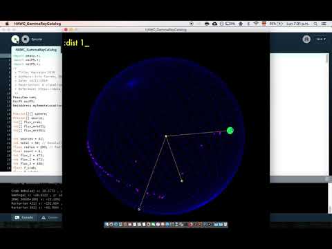
The pictorical representation is a reconstruction of 39 gamma-ray sources from 2nd HAWC observatory catalogue, mapped into a 3D computer-based visualization of a spherical coordinates system. That might (I hope) been integrate, in the future, and as many as possible, with mostly all of the aspects from the phenomenon –like in a quantum resolution, perhaps–, from the prototypes developed in the Astronomic Hackathon 2018, and with UNAM's Astronomy Institute, Dr. Magda González, Sergio Hernández, and the founders of the summon Carles Tardío, Rodrigo Treviño, Leslie García and everyone who were involved in the support of the project.
The audio representation is a reconstruction of a 472 flux transitions from Lightcurves of Crab Nebulae, Markarian 421, and Markarian 501, mapped into three differents synths...
The process, which describes the implementation of the prototypes, starts as follows:
In the first day, we were summoned by Art, Science, and Technology's (ACT) program in the wild México City to attend a series of talks and workshops at UNAM's Astronomy Institute headquarters during the 6th, 7th, and 8th of november from 10-14h and from 16-18h.
We were introduced to the observatory, and physics foundations with a talk from Dr. Magda González about Cosmic ray as a messengers from the universe, to adapt our thoughts to the domain language.
Most of chemical elements that represent Mendeleev's periodic table comes from out of the earth. In fact, certain elements have been produced by the human being activity.
So we ask ourselfs, from where the hell comes all the matter?!
 |
 |
 |
In a modern vision way, the fundamental particles, viz., quarks, electrons, neutrinos, muons, taus where ionized during the cooling and the acecelerate expanse of the universe since the Big bang. Once that these particles became with a more complex structure, because of gravity, heat and many other stuff, the first stars and galaxies started to bright.

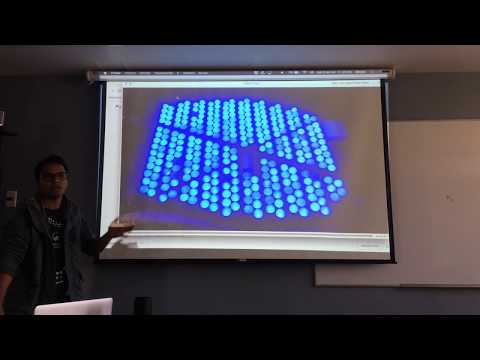
After that, we jumped into a laboratory where they explained us how does it work, in general, the electronic system of the HAWC's Observatory. The most interest part, from my point of view, is when the Cherenkov's effect lights the photocathode in the tubes to photomultiply it into many electrons, which sends a signal to the engineering mechanisim, where a front-end board recieve these pulses and translate them into bitcode, and then process it with another machines-levels to get the data in a natural language.
 |
 |
 |
 |
Next, we were on an underground laboratory where they showed us the purified quality water process of the modules, with a laser passing through a tube filled with dirty water.
 |
 |
 |
At the end of the day, we had a nice exploration of the first Data Sets with Sergio Hernández, whom facilitated us the reading for each of the sets' parameters. For example, the 39 Gamma-Ray sources that allow them to plot the sky, or the maps from the observation significance of each source, or the lightcurves from Crab Nebulae, Markarian 421, and Markarian 501 from about 17 measuring months.
Note: The format of the data files is very important for the implementation of the project. In this case, the second catalogue is in .xml file, but Sergio provided us a program to convert it to .csv with python. The lightcurves are in .dat file, so with a kind actitude from my friend Emmanuel, we could solved the problem to reconstruct the data in a readable format for the environments that we wanted to use. There was a interested fact in the variables of this set, that Sergio helped us with the dates in which the transition from the fluctuation started and stopped recording. by converting the Modified Julian's Calendar to Gregorian's Calendar with some tricks from the Astropy.time module.
Now, we were ready to ping some ideas with the community!
 |
 |
 |
Finally, the mentors assigned to the mission, presented their portfolios with conceptual tools from the paradigms of programming languages, like; SuperCollider, Pure Data, VVVV, OpenFrameworks, and Processing. Which it is intended to specify this aspect forward.
In the second day, we started in the cafeteria's 2nd floor in the Astronomy Institute to share some ideas, with different points of view for what is supposted to be the final reconstruction from what we heard and felt previously. As a group whom starts a problem since the beginning, we decided to present it for the International Night's Stars Festival on 17th of november in differents resolutions or scales: as a main in the interstellar medium, as a pre cascade in the earth's atmosphere and post cascade in the HAWC Observatory, and as a particular periodistic way.
 |
 |
 |
In this photo my name appear with 'k' instead of 'c' and with '?', because at that time of the day I had to leave early the meeting. But definitely, I was agree with the idea about mapping the 39 gamma-ray sources using the galactical coordinates from the catalogue, because I decided to share with the community a sketch in which I'm recenlty working for my master's degree. And also, I was interested in the work proposed by Emilio and Marianne, about sending values through an Open Sound Control (OSC) Protocol cause it is a nice solution to integrate the work of everybody in a single presentation.

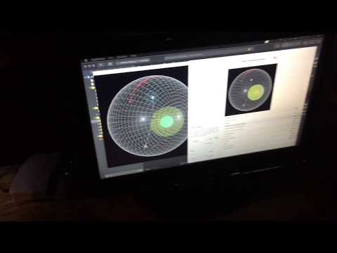
In the third day, we were ready to begin to synthetize the data. But first, we need to realized some speculative details about the sequence of time, in which the cascade takes roll in every module of the observatory. For that reason, Sergio shared with us a model that reconstructs the events in a longer scale of time.

 |
 |
 |
Now, I propose a guide which could probably help or agile the winnings for the project:
1.1. Determine which variables from the tabular representation we need use to answer what we are looking for.
Note: the data is recolected from the electromagnetic pulse which sends the PMT floating in every single one of the modules.
- Name of the celestial source.
- Galactical, ecuatorial and spherical coordinates.
- Distance of the object in parsecs.
- The transitory amplititude from the fluctuation of the Crab Nebulae, Markarian 421, Markarian 501.
- Position of the camera inside the simulation.

We had the opportunity to reach Carles and Sergio knowledge by explaining the meaning of galactical coordinates, and how to transformed them to a spherical system, with again, some tricks from the Astropy module.
We commonly agreed in define 200 parsecs of distance.


We need to reconstruct the tabular representation from the .dat file to export it to .csv. Thanks again to Emmanuel for his help!


At the beginning, we had some troubles for shooting the .csv files, because of the way we need to call them in every environments.Then we needed to parse and assign them to the right data type. But we solved it!


In my case, I wanted to represent the amplitude fluxtuation from the sources by moving the strokeWeight's parameter depending from the values in the datasets. So, it is a good idea to integrate the local reconstructions by receiving a set of values from another platform through this protocol, which use the NetAddresses from the local devices to interchange data.
    OscP5 oscP5;
    NetAddress myRemoteLocation;

    float f_crab;
    float f_mrk421;
    float f_mrk501;
    String typed = "";

    void setup() {
        /* Start oscP5, listening for incoming messages at port 12000 */
        oscP5 = new OscP5(this, 12000);

        myRemoteLocation = new NetAddress("127.0.0.1", 12000); // Local
        //myRemoteLocation = new NetAddress("192.168.1.100", 5612); // Emilio
    } //------------------------------------------------------------------------------------------------------ setup

    void draw(){
      /*
       * Draw
       * GAMARAY SOURCES
       * – pulsar, super nebulae, star collision, galaxy centers –
       */
      for (int i = 0; i < source.length; i++) {
        PVector v1 = source[i]; // PVector
        //----------------------------------------- The Sun at the center in color white
        stroke(255, 255, 0);
        strokeWeight(7);
        point(0, 0, 0);
        if (i == 1) { //--------------------------------------------- Draw Crab Nebulae
          stroke(random(255), random(255), random(255));
          strokeWeight(int(f_crab*5000));
          //strokeWeight(flux_crab[int(random(flux_crab.length))]);
          point(v1.x, v1.y, v1.z);
        } else {
          if (i == 7) { //------------------------------------------- Draw Markarian 421
            stroke(random(255), random(255), random(255));
            strokeWeight(int(f_mrk421*5000));
            //strokeWeight(flux_mrk421[int(random(flux_mrk421.length))]);
            point(v1.x, v1.y, v1.z);
          } else {
            if (i == 9) { //----------------------------------------- Draw Markarian 501
              stroke(random(255), random(255), random(255));
              strokeWeight(int(f_mrk501*5000));
              //strokeWeight(flux_mrk501[int(random(flux_mrk501.length))]);
              point(v1.x, v1.y, v1.z);
            } else { //-------------------------------------------- Draw the rest of the sources
              stroke(random(255), 0, 255);
              strokeWeight(6);
              point(v1.x, v1.y, v1.z);
            }
          }
        }
    } //------------------------------------------------------------------------------------------------------ draw

    void keyPressed() {
      if (key == ENTER && typed.equals("3")) {
        /* in the following different ways of creating osc messages are shown by example */
        OscMessage myMessage = new OscMessage("/fuente");
        myMessage.add(3); /* add an int to the osc message */

        /* send the message */
        oscP5.send(myMessage, myRemoteLocation);
      }
    } //------------------------------------------------------------------------------------------------------ keyPressed

    /* incoming osc message are forwarded to the oscEvent method. */
    void oscEvent(OscMessage theOscMessage) {
      /* parse theOscMessage and extract the values from the osc message arguments. */
      if (theOscMessage.addrPattern().equals("/crabSend")) {
        f_crab = theOscMessage.get(0).floatValue();
        //println("### values from /crabSend pattern: "+f_crab);
      } else {
        if (theOscMessage.addrPattern().equals("/mrk421Send")) {
          f_mrk421 = theOscMessage.get(0).floatValue();
          //println("### values from /mrk421Send pattern: "+f_mrk421);
        } else {
          if (theOscMessage.addrPattern().equals("/mrk501Send")) {
            f_mrk501 = theOscMessage.get(0).floatValue();
            //println("### values from /mrk501Send pattern: "+f_mrk501);
          }
        }
      }
      int firstValue = theOscMessage.get(0).intValue();
      println("\n### values from the osc message: "+firstValue);
      /* print the address pattern and the typetag of the received OscMessage */
      //println(" typetag: "+theOscMessage.typetag());
      println("### received an osc message. with address pattern: "+theOscMessage.addrPattern());
      println("### IP address: "+theOscMessage.address());
      println("### port: "+theOscMessage.port());
      println("### NetAddress: "+theOscMessage.netAddress());
    } //------------------------------------------------------------------------------------------------------ oscEvent
The OSC Protocol works by defining three patterns or tags, like /crabSend, /mrk421Send, and /mrk501 to send messages or data. In this case, the data came in string type so I had to parse them to float to use it in the way I needed.
 |
 |
4. Implement an Interactive User-Interfaced to control the exploration of the visualization (pending).
There were certain suggested technology tools to handle the challenge for the project. Meanwhile, some were interested in visualize the phenomena, and some were in sonorize it too. For that reason, I decided to visualize it by using a graphic library based on Java programming language in an platform call Processing, and the data analysis I used the environment Jupyter Lab for develop Python language.
The rehearsal took place at Los catorce 14 two days before the presentation. We had the chance to critize our prototypes with a video projector and sound system. Just to get in touch with the rest of the work and how we were gonna organize the whole performance.
One of the ideas that I took from Emilio and Marianne, was about the experience that they have to get in mind all the needs, requirements, and all the equipment that must be move from our places to the forum or stage. It was a quite single!


It was the day! The team decided to test some specific aspects for the live coding performance for having it ready at time. The presentation took place at Las Islas in Ciudad Universitaria (UNAM) at 18h beside the main stage. It were a nice weather, and the crowd were satisfied!

 |
 |
 |

- datasets/Hackaton2018.ipynb: Data analysis with python.
Some docs from Astropy module that were used:
- visualization/HAWC_GammaRayCatalog/HAWC_GammaRayCatalog.pde: Data visualization with Processing.
To adapat the strokeWeight of the sources Crab Nebulae, Markarian 421 y Markarian 501 to the OSC messages from SuperCollider, setup the port as follows:
Orb.start("192.168.1.111", 12000); // la dirección de la otra compu. Se necesita la librería PiranhaLab
Then comment and uncomment the next lines in the Processing code:
strokeWeight(int(f_crab*1000));
/strokeWeight(flux_crab[int(random(flux_crab.length))]);

strokeWeight(int(f_mrk421*1000));
//strokeWeight(flux_mrk421[int(random(flux_mrk421.length))]);

strokeWeight(int(f_mrk501*1000));
//strokeWeight(flux_mrk501[int(random(flux_mrk501.length))]);
Now, you can run the app while SuperCollider is running too!
https://es.wikipedia.org/wiki/Fotomultiplicador
http://artecienciaytecnologias.mx/
https://www.hawc-observatory.org/
https://historiaybiografias.com/calendario/
https://www.nochedelasestrellas.org.mx/
http://www.astroscu.unam.mx/IA/index.php?lang=es
https://en.wikipedia.org/wiki/Cherenkov_radiation
Hernández, Sergio. (2018). El Observatorio HAWC. Instituto de Física, UNAM: México.
Hernández, Sergio. Data Sets I
Marciniak, Ryan. (2016). Where did the Elements Come From?